

TLDR
- Causal graphs are a key element of correct causal modelling and can be created with causal discovery techniques or domain knowledge.
- All causal graphs can be decomposed into three-node building blocks: chains, immoralities, and forks.
- Simple causal analysis can resolve complex paradoxes such as the Berkson's and Simpson's paradoxes.
Welcome back to the second installation of our introduction to causal inference series! In part one, we explored the motivation behind causal inference and the importance of causal relationships, so make sure to check it out here if you haven’t already.
In this part, we will learn all about simple causal graphs and we'll use them to resolve some of the well-known paradoxes in statistics.
Importance of causal graphs
It's impossible to form an estimation of causal effects without knowing how variables interact and this is the vital piece of information reflected in causal graphs.
But what is a causal graph?
A causal graph is a representation of the data that gives deeper understanding into the causal relationships hidden within. They can be based on causal discovery methods which estimate causal links using observational data. Alternatively, one may use domain knowledge to construct it. Once we have a causal graph, the estimation of causal effects relies on how we adjust correctly for variables that introduce false associations.
To fully understand the structure of causal graphs and how the adjustment procedure may work, it is worth discussing the “building blocks” of causal graphs. The focus in this article will be chain, immorality, and fork building blocks [1]. Whilst other types of building blocks do exist - namely two connected and two unconnected nodes - we can consider these as trivial in relation to casual graphs and will be ignored in this article.
Chain
This building block represents a relation of the type A → B → C, where B is called a mediator. An example is the process of fire causing an alarm activation [1]. Alarms are actually triggered not by fire but by smoke molecules blocking an LED light stream which the detector registers as a scattering of light. In other words, smoke mediates the causal effect of fire.
Could we claim that fire does not cause the alarm? No, it would be wrong. The total causal effect consists of a direct and indirect causal effect. If there is a causal path between two variables, then a causal effect is present.
A causal path between X and Y is a sequence of nodes and edges starting from X and finishing at Y where all edges point in the same direction (i.e. a directed path between X and Y).
Fire does not have a direct causal effect on alarm because it is not its "parent". The implication is that conditioning on smoke (i.e. knowing its value) makes information about fire useless. Nonetheless, the smoke has a non-zero total causal effect on alarm since there is a causal path coming through the mediator which introduces an indirect effect.
Immorality and Berkson’s paradox
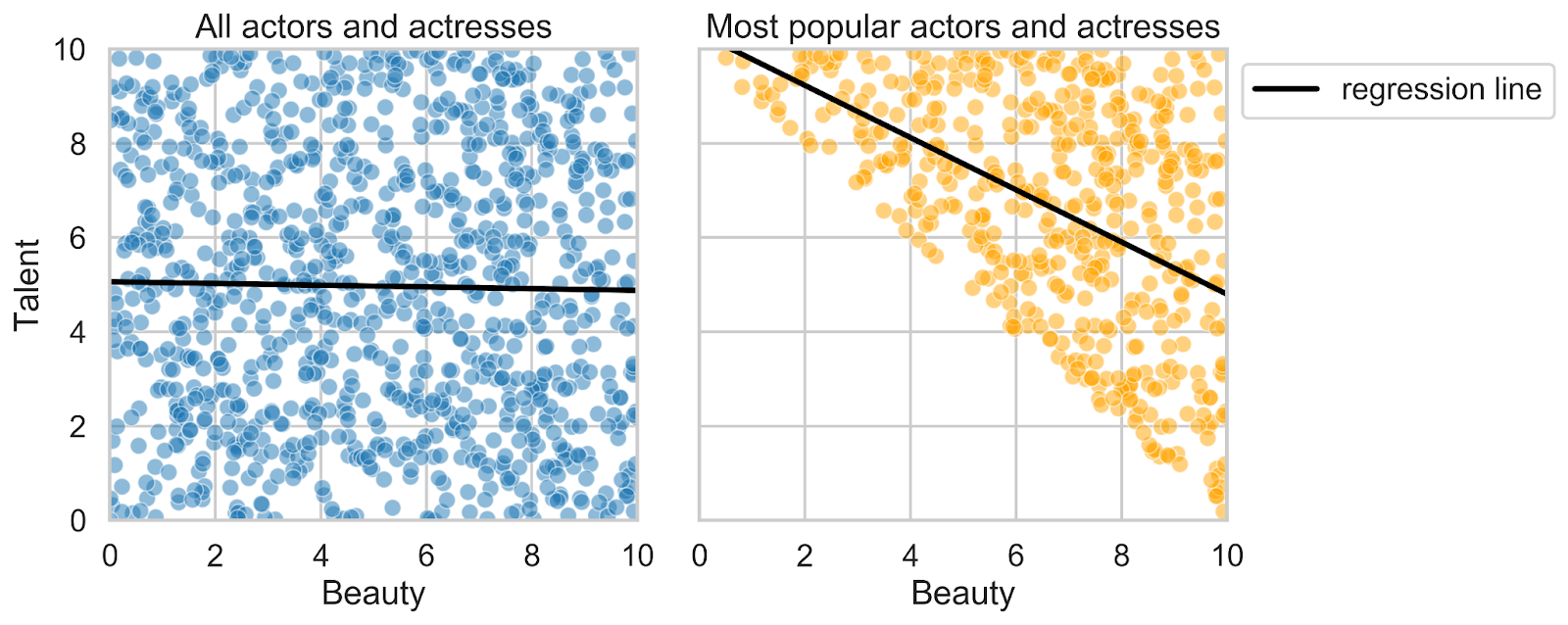
Yes, "immorality" is a real scientific term and it denotes the junction where two variables cause another one: A → B ← C. In this instance, variable B is called the collider and A and C are assumed to be independent. Consider a fictional (although perhaps not remote) world in which talent and beauty are the two facts that determine the celebrity level of Hollywood stars [2]. Assume we rate all actors and actresses from 0 to 10 and their popularity level is the average of the two. Figure 1 demonstrates the distribution of the corresponding data. Looking at the entire sample of actors and actresses, we see no relation whatsoever between skill and appearance (the left-hand side plot). However, if we focus on the most popular stars, beauty and talent become strongly negatively correlated. This phenomenon is called Berkson’s paradox or a collider bias.
Our knowledge of the underlying causal graph tells us that this negative association is spurious. The biased non-zero correlation has been introduced by conditioning on popularity, that is, by considering a stratum of very famous stars. Intuitively, the bias occurs because it is usually sufficient to be exceptionally talented but have a modest appearance to be a superstar, and vice versa. That is, one of the features tends to “explain away” fame. To estimate the causal effect between beauty and talent correctly, no conditioning is needed.
Fork
The previous article in this series provided an early entry into the notion of forks in casual inference. This junction takes the form A ← B → C. B in this case is known as the confounder. As you may remember, confounders introduce a bias into a causal effect estimate between A and C. To eliminate this bias, we need to condition on a confounder.
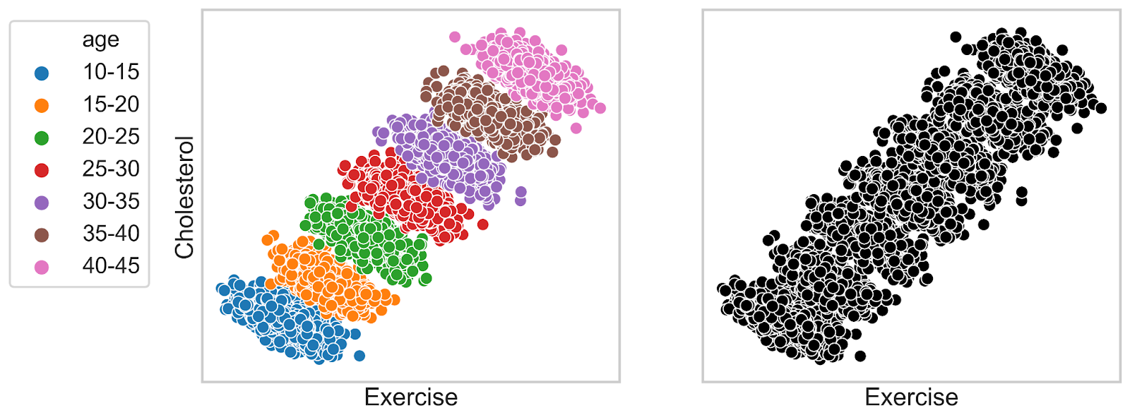
Suppose we arrived in an alternate universe where people tend to exercise more frequently as they get older. However, there is a positive relation between age and cholesterol. After gathering data on those people we plot Figure 3. If we segment observations by age, physical activity and cholesterol are negatively associated. In contrast, if we look at the population as a whole, exercise has a detrimental (positive) effect on cholesterol and thus increases the chances of heart diseases. Well, should we recommend those people to quit sports?
No, we should not, and we can prove this by looking at the causal structure related to the variables. Age is not caused by any of the two other variables and increases the level of cholesterol. Since older inhabitants prefer exercising more, age causes exercise on that planet. Therefore, the relations are represented by the fork "exercise ← age → cholesterol", where age turns out to be a confounder. Therefore, to estimate a correct causal effect of sports on cholesterol we need to condition on age. After doing this correction, we reaffirm the beneficial effect of exercise on the level of cholesterol. This beneficial relationship can be seen within any individual coloured segment in figure 2 (more exercise lowers cholesterol).
Conclusion
A causal graph is an essential starting point of any causal effect estimation. Understanding which parts of the graph can introduce spurious association is vital for appropriate bias correction. We have seen how we can resolve some of these biases (a.k.a. paradoxes) using causal diagrams.
In the next series, we will discuss how to deal with larger causal graphs to estimate causal effects, so stay tuned!
*Disclaimer - All views in this article belong to Maksim Anisimov and are not a reflection of his employer or wider affiliations.*
References
[1] Judea Pearl and Dana Mackenzie. 2018. The Book of Why: The New Science of Cause and Effect (1st. ed.). Basic Books, Inc., USA.
[2] Elwert, Felix & Winship, Chris. (2014). Endogenous Selection Bias: The Problem of Conditioning on a Collider Variable. Annual Review of Sociology. 40. 31-53. 10.1146/annurev-soc-071913-043455.