

Worldwide, the scientific community and beyond has become remarkably conscious of the importance of Data Science, AI, Machine Learning (ML), Neural Networks and their numerous applications. However, having browsed thousands of different learning platforms, participated in data science challenges and attended multiple quant webinars, I have concluded that only a handful of those practitioners who claim to use AI/ML actually have an understanding of the underlying principles; aka the black box approach. Without a full picture, one can only wonder what the outcomes will be. This intro to Machine Learning article series aims to reconcile this problem by giving a basic insight into the inner machinery of ML. In doing so, I hope to equip you with the skillset to ask the right questions when utilising AI or ML algorithms.
I joined the data science community this summer when I first started diving into the world of finance and hence cannot claim myself to be a know-it-all in this complex data world. However, what I can offer to the Nural readers is my determination and will to comprehend the ML algorithms. The series will be an in-depth analysis of the theory behind each class of algorithms in the context of climate change and medicine. We kick off with Linear Regression.
Machine Learning in brief
At its simplest, machine learning (ML) is curve-fitting given a certain optimisation algorithm, i.e. getting a model to accurately describe data points where the optimisation algorithm let’s the machine know how well it has done.
Carnegie Melon University professor, Tom Mitchell describes the process as follows – “A computer program is said to learn from experience E with respect to some task T and some performance measure P, if its performance on T, as measured by P, improves with experience E.” The following flow chart represents a general idea behind ML:
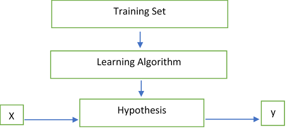
Looking at the figure above, the question that ML answers is: How do we best represent the relationship between our inputs "X" and our outputs "y", aka the hypothesis function h(X)? These inputs and outputs could be as simple as trying to find the relationship between age and likelihood to take an afternoon nap!
For this introduction, we will start with the most basic type of relationship between y and x: a linear relationship. The below section is a bit maths heavy, if that isn't for you then skip over it for the summary in context.
This leads us to the linear regression model which in mathematical notation is as follows:
$$h(x) = \theta_0 + \theta_1 X$$
For the more advanced this can be rewritten as below (where n is the number of features)
$$ h(x) = \Sigma_{i=0}^{n}\theta_i X_i$$Throughout the series, I will adhere to the Stanford University notation as per below:
|
q |
m |
X |
y |
(X, y) |
n |
|
Parameters to optimise |
# of training examples |
Inputs/features |
Output/targeted variable |
Training example |
# of features |
Back to linear regression
Now we have all of the fancy notation out of the way, we can focus back in on linear regression. The aim of ML is to find the relationship between an input and an output and linear regression assumes that the relationship can be modelled using a straight line. This is a supervised learning algorithm as to train it, we must provide the inputs as well as the expected outputs. Below are some key points relating to linear regression.
- Regression means a problem requiring fitting any kind of model into any kind of data.
- Regression assumes that the targeted variable is continuous.
- Regression does not have to be linear; it can be any function you can think of, quartic, exponential, logarithmic.
- Note that no phenomenon in the world is purely linear; there are no objects/natural forces that interact with each other in a strictly linear way. Hence, one of the limitations to consider when creating a model hypothesis is something known as underfitting or what ML professionals call 'model bias'.
Optimisation algorithm
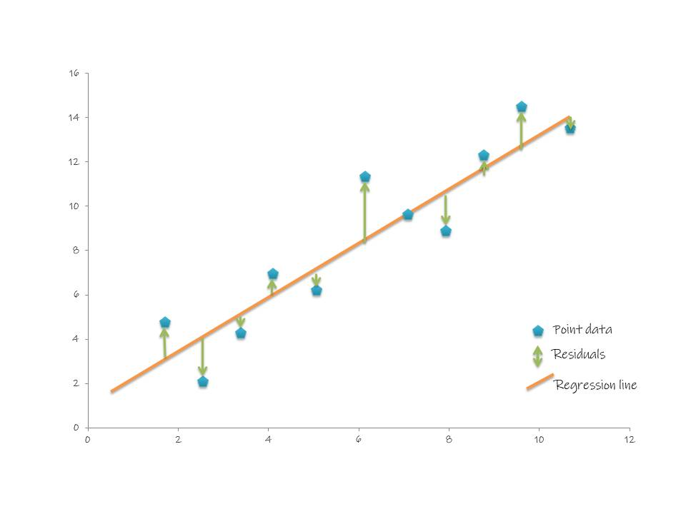
We started by outlining that machine learning fits a curve (or in this case a straight line) by using an optimisation algorithm where the optimisation algorithm is a function that minimises what's known as a cost function "J(θ)". In the case of linear regression, the cost function is the sum of squared residuals/ mean squared error (MSE) and this function lets us know how well the model has fit onto the data points. The graph above demonstrates what a residual is in the context of a linear regression line. The MSE finds the squared distance between the line and the actual data point for a given value of x. In mathematical notation:
$$MSE = \Sigma_{i=1}^m(h(x)-y)^2 *0.5$$
The actual algorithms for minimising the MSE are under a methodology known as gradient descent and we will dive deeper into this in the coming months. Fortunately, Python packages make this easy to implement in practice.
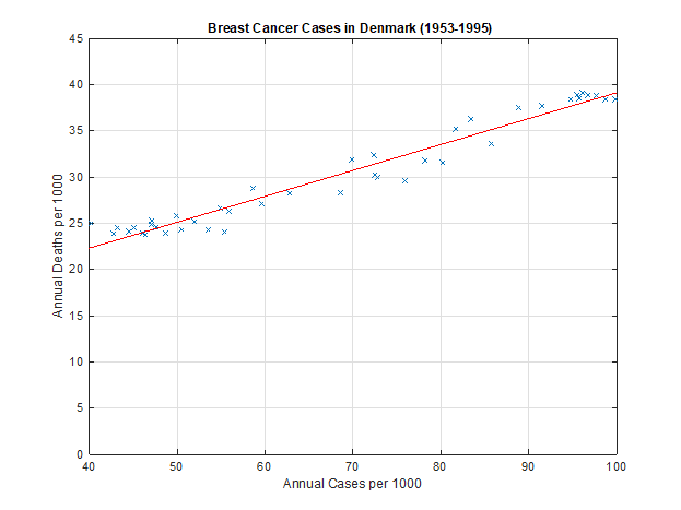
Equipped with the architecture for linear regression as well as the cost function which must be minimised using optimisation algorithms, the linear regression line can now be fit onto the a real life dataset. This has been done below to model breast cancer cases in Denmark.
Conclusion
What's been covered in this first part of this series:
- You've learnt that machine learning is simply curve-fitting given a certain optimisation algorithm
- You've been introduced to the first supervised ML technique: Linear Regression
- You've learnt that for linear regression, the MSE function must be optimised to fit the line to the data points!
Later in the series I will go into bringing this to life using Python alongside other more complicated ML techniques such as Neural networks.