

Dear followers, welcome back to the third instalment of the intro to ML series! In this edition, the ultimate aim is to demonstrate how we can arrive at some of the conclusions we had previously learnt, but by taking a probabilistic approach instead. If you recall, the core of the machine learning process constitutes optimisation of a cost function. This same cost function will be derived but this time using the principle of maximum likelihood. P.S.: If some of the mathematical notation looks overwhelming, don’t worry! You will still be able to follow along from just the text.
If you missed the previous parts in series, or you just want to get some familiarity of what we are discussing, then make sure to check out part 1 and part 2.
Let's Begin
Before diving into the derivation, we must first build out the following two assumptions about the nature of the data that we are working with.
Assumption #1
Assume that the target variables y and the inputs x are related via the equation
$$y^{(i)} = \theta^Tx^{(i)} + \epsilon^{(i)} (1)$$
where ϵ(i) is a random error, or in ML terms- 'unmodeled' effects. The associated effects are pertinent to the model, but we did not account for them or merely could not account for them due to lack of knowledge. For instance, a malignant breast tumour linear regression model that does not consider a patient's age exemplifies the case where epsilon would be high due to unmodeled effects.
Assumption #2
Another assumption to take on board is that epsilons are Gaussian IID (independently and identically distributed). To give you an example, successions of throws of a fair coin are IID because:
1) The coin has no memory, i.e. your chances of throwing heads or tails are the same on every iteration (hence independent)
2) Every throw is a 50/50 chance and the probability distribution does not change (hence identical)
Now let’s dive into it
Let’s recall what Gaussian distribution (aka normal distribution) look like.
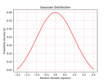
Gaussian distribution is characterised by two constant parameters- mean (μ) and variance (σ^2) and in mathematical notations written as
ϵ ~ N(μ,σ2)
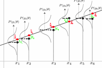
This Gaussian/ normal distribution turns out to be very important as we assume that the error is distributed normally with a mean of zero and variance of σ2. However, we can also assume that each y(i) or observation is distributed normally with a mean of θT x(i) and a variance of σ2 as seen in equation 1 (see figure 2 for a graphical representation).
So what’s our aim?
Ultimately our aim is to find the value of theta that maximises the chance of seeing our observations y given our input data x. The normal distribution is well known and equation 2 houses the probability of seeing an observation y given our input data x and parameters (in case you struggle with normal distributions, this link will help you get up to speed).
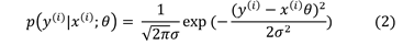
This formula above is the PDF. We, diligent statisticians, want to know what is the probability of seeing a y(i) given by x(i), parametrised by θ (equation 1). This question implies that y(i) is a function of x(i) for some constant theta, but that is not what we are after. We want θ to be variable and x(i) to be controlled, right? x(i) is controlled as these are the fixed data points we are given.
Therefore we look for methods to maximise the chance of seeing data giving a certain value of theta. The explicit name for such probabilities is- likelihood! You will hear this word a lot amongst ML users and all it means is the probability of seeing certain outputs, given the chosen parameters theta. Because of the independence assumption on epsilon and on y, the likelihood of theta is merely the product of all such probabilities, i.e. take the equation (2) and multiply the probabilities out for every observation in your data.
Lastly, to ensure we choose the right theta, we need to maximise the likelihood (aka principal of maximum likelihood). In other words, we choose theta to make the data as high probability as possible. Instead of maximising the function L directly, we can maximise the log of L, and after some manipulations, we arrive to
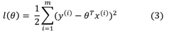
which is exactly what we prescribed to the cost function J in previous parts of the series (full derivation)! Interestingly, the maximum likelihood function is independent of unmodeled error spread and can be found directly from your data.
Conclusion
The parameters of a linear regression model can be estimated using a least squares procedure or by a maximum likelihood estimation procedure. Now you have become a noticeable linear regression practitioner who understands the underlying assumptions of this commonplace algorithm. You are prepared to unlock the full potential of linear regressions, good luck!