

TLDR
- Linear regression is a type of supervised learning algorithm
- The aim of ML is to fit the linear regression coefficients to the dataset
- The normal equation is a method of fitting the equation to the dataset
We're back with the second in our introduction to ML series where we are exploring major axioms with the ML world to make it accessible to all. Last post, we looked at how ML looks to predict the future by looking at historical data and optimising a function to fit the data. We then first came across linear regression (y = mx + c) and how we can fit this straight line to a dataset using gradient descent.
In this post, we'll be continuing our exploration of linear regression and explore one of the most important equations in the world of machine learning- The Normal Equation.
Why is the normal equation important?
Linear regression is a supervised machine learning algorithm which can be represented as:
$$y(x) = \theta_0 + \theta_1 X$$
|
q |
m |
X |
y |
(X, y) |
n |
|
Parameters to optimise |
# of training examples |
Inputs/features |
Output/targeted variable |
Training example |
# of features |
The aim of linear regression in machine learning is to find the values of theta which will accurately describes the relationship between the inputs and the outputs. The normal equation obtains these theta coefficients and this is why the equation is so important.
Let's ground this with an example
A gentle reminder that a supervised algorithm is an algorithm where it learns from previous examples. The algorithm will be fed a labelled training set to learn from and then go on to predict on unlabelled test data.
For instance, in the context of climate change if one wants to predict emission per in a given region, a useful set of training labels can include:
- Number of factories per km2
- Number of cars per household per km2
- Urban population per km2
- Building energy intensity
As a data scientist, you would collect these features and record an associated value of CO2 emission per km2. Note that because each of the four features is associated with a specific CO2 value, the machine learning algorithm can be classified as 'supervised'. Also note that because we have four different variables, the algorithm would be called Multivariate Linear Regression. Multivariate means to have multiple variable/features within your model. The resulting multivariate linear regression equation becomes:
$$y(x) = \theta_1 x_1 + \theta_2 x_2 + \theta_3 x_3 + \theta_4 x_4$$
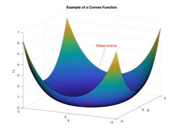
Theta coefficients that yield global minima should be taken as the 'optimal' parameters. Now, here is a trick! Typically one would have to iterate over a set of theta values using batch or stochastic gradient descent (as described in the last edition), but the coefficients of linear regression can be obtained using the normal equation.
Deep dive into the Normal Equation
Mathematical notation for normal equation: $$\theta = (X^TX)^{-1}X^Ty$$
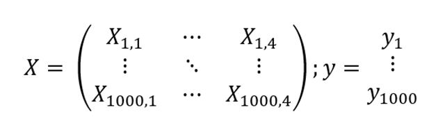
The above elegant equation is called "Normal Equation" (full derivation). Let me now walk you through the meaning and technicalities of the equation above. X is a vector containing our four features, where each row and column correspond to an observation and a feature, respectively. If, for instance, you were to record data about 1000 different locations independently, then your matrix X would have 1000 rows and 4 columns. Vector y would simply be the recorded data points of CO2 emission per km2.
Here is a caveat, we have not yet considered an intersection! Remember the equation of line y=mx+c? We defined matrix X to take four features, i.e. there will be four allocated feature values m1, m2, m3, m4 but what if at X_0=[0,0,0,0] we have a non-zero value of y? In our example, CO2 emission would not be equal to zero at X0 because the Earth's atmosphere by default has some amount of CO2 particles, so having an intercept is a must. We can then rewrite X as with 1000 rows and now five (4+1) columns, where the last column is filled with dummy values of 1's. Hence, for a single observation, our equation for X would be as follows:
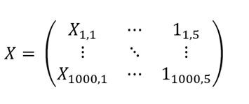
Introduction of a dummy variable enabled us to account for an intercept with the y-axis.
Back to the normal equation, XT indicates a matrix transpose and (XT X)-1 means inverse of a matrix. To wind up this topic, let us finally perform a sanity check on the matrix dimension we obtain from the elegant equation above.
$$((5×1000)×(1000×5))×((5×1000)×(1000×1))=(5×1)$$
Hence, theta is a (5x1) vector, just what we needed! With these five coefficients, you can now predict the CO2 emission based on the four features you observe.
Conclusion
Don't worry if the mathematical notations looked ambiguous to you, running a linear regression code yourself will certainly help! For this reason, I have created a Python script which you can run using PyCharm or Jupiter Notebooks. Remember, practice makes perfect; the more you use linear regression in daily life problems, the more comfortable you will become with the notations and technicalities!